Bottles and Cans
Seinfeld: S7, E21–22 “The Bottle Deposit”
Production and Costs: Average Total Cost
(Based on an original idea by Eduard Levin, a student at the University of St. Thomas)
Kramer won’t throw away a bottle that could be recycled. He wants the five cents that New York will pay for each bottle turned in. Newman, who has just found out about the bottle deposit system, learns that Michigan is more generous: ten cents a bottle.
Newman: “Wait a minute. You mean you get five cents here, and ten cents there. You could round up bottles here and run them out to Michigan for the difference.”
Kramer: “No, it doesn’t work.”
Newman: “What d’you mean it doesn’t work? You get enough bottles together...”
...
Newman: “You tried it?”
Kramer: “Oh yeah. Every which way. Couldn’t crunch the numbers. It drove me crazy.”
Why don’t the numbers crunch the way Kramer wants? Sure, five extra cents for each bottle is not much. But there must be some number of bottles large enough to make a run to Michigan profitable as opposed to depositing locally.
This is an example where thinking carefully about costs comes in handy. Let’s crunch the numbers ourselves over possible quantities of bottles.
This potential scheme involves two types of costs. Fixed costs don’t increase or decrease as Newman and Kramer haul varying quantities of bottles. It makes no difference whether they run 1,000 bottles or 10,000. Fixed costs are fixed. They’ll need to rent a vehicle. A trip to Michigan will burn lots of gas.11 By listing gas as a fixed cost, we’re assuming the bottles are light enough to have no noticeable effect on gas consumption. There may also be lost wages from the trip if Kramer and Newman must forgo work or another promising scheme.
Variable costs increase as the quantity increases. Fitting more bottles into a vehicle gets tricky as it nears capacity. This will take valuable time and energy. These costs show up in marginal cost: the added cost from transporting one more bottle.22 Marginal cost is the change in total cost from one more bottle. Since fixed cost doesn’t change with additional bottles, marginal cost reflects only changes in variable cost. Mathematically, marginal cost is the derivative of either total or variable cost with respect to quantity. Because variable cost rises faster at high quantities, marginal cost (eventually) increases as the number of bottles grows.
Why doesn’t a bottle run to Michigan look profitable?33 By profit, we mean economic profit, which accounts for opportunity costs. Their scheme could turn an accounting profit without being better than the next-best use of their time. Kramer and Newman need their total cost from the trip to be below their total revenue. In this case, we can model revenue as $0.05 multiplied by the number of bottles run to Michigan. It’s the difference between the Michigan price and the New York price. A negative profit implies that they would do better to deposit their bottles in New York than in Michigan.44 Alternatively, one could model this with the two receiving $0.10 for each bottle in Michigan. The $0.05 they could have received in New York is then added to marginal cost for every bottle transported. The conclusions would be identical.
Equivalently, profitability means getting average total cost below $0.05, where average total cost is total cost divided by quantity. If, on average, each bottle costs less than $0.05 to transport, they come out ahead.55 Why relative to average total cost and not average variable cost? They don’t have a truck yet, so their fixed costs are not sunk.
At very low quantities, average total cost will be remarkably high. Imagine how costly it would be, per bottle, for the two to transport one bottle to Michigan. But as they expand, average total cost will fall as fixed cost gets spread over higher quantities, and variable cost has yet to get out of hand. At some point, marginal cost will cross average total cost, and at every quantity beyond that point, average total cost will increase with quantity. The scale of the operation gets away from them.
The graph below visualizes this relationship and shows that the scheme has no chance, at least with a pickup truck.
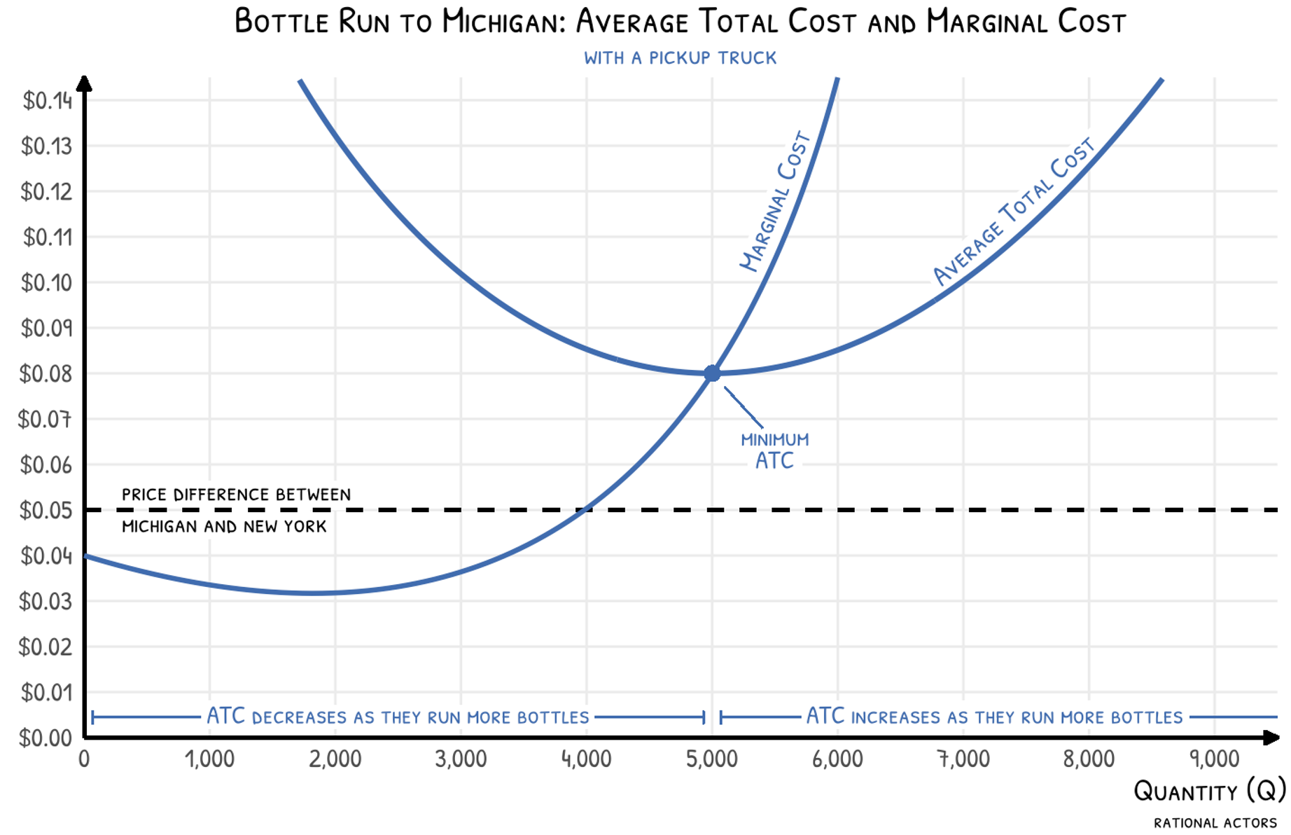
The lowest average total cost the operation can achieve with a pickup truck is $0.08. The numbers don’t crunch because of the fixed cost. The first 4,000 bottles all have marginal costs below $0.05, so those bottles pay for their own loading. But they can’t get the fixed cost covered before space runs short.
They need new ideas. Maybe a vehicle that can handle a bigger load would keep the marginal costs down over a much greater quantity. That might do the trick.
Newman: “I don’t understand. You fill an eighteen-wheeler?”
Kramer: “No, an eighteen-wheeler’s no good. Too much overhead. You got permits, weigh stations, tolls. Look, you’re way outta your league.”
As Kramer points out, the big truck comes with additional fixed costs. They may end up carrying a lot more bottles but be no closer to profitability.
Newman: “So, we could put the bottles in a U-Haul. You know, go lean and mean?”
Kramer: “Newman, it’s a dead end, c’mon.”
Each vehicle has its own average total cost curve, and we can plot them together.
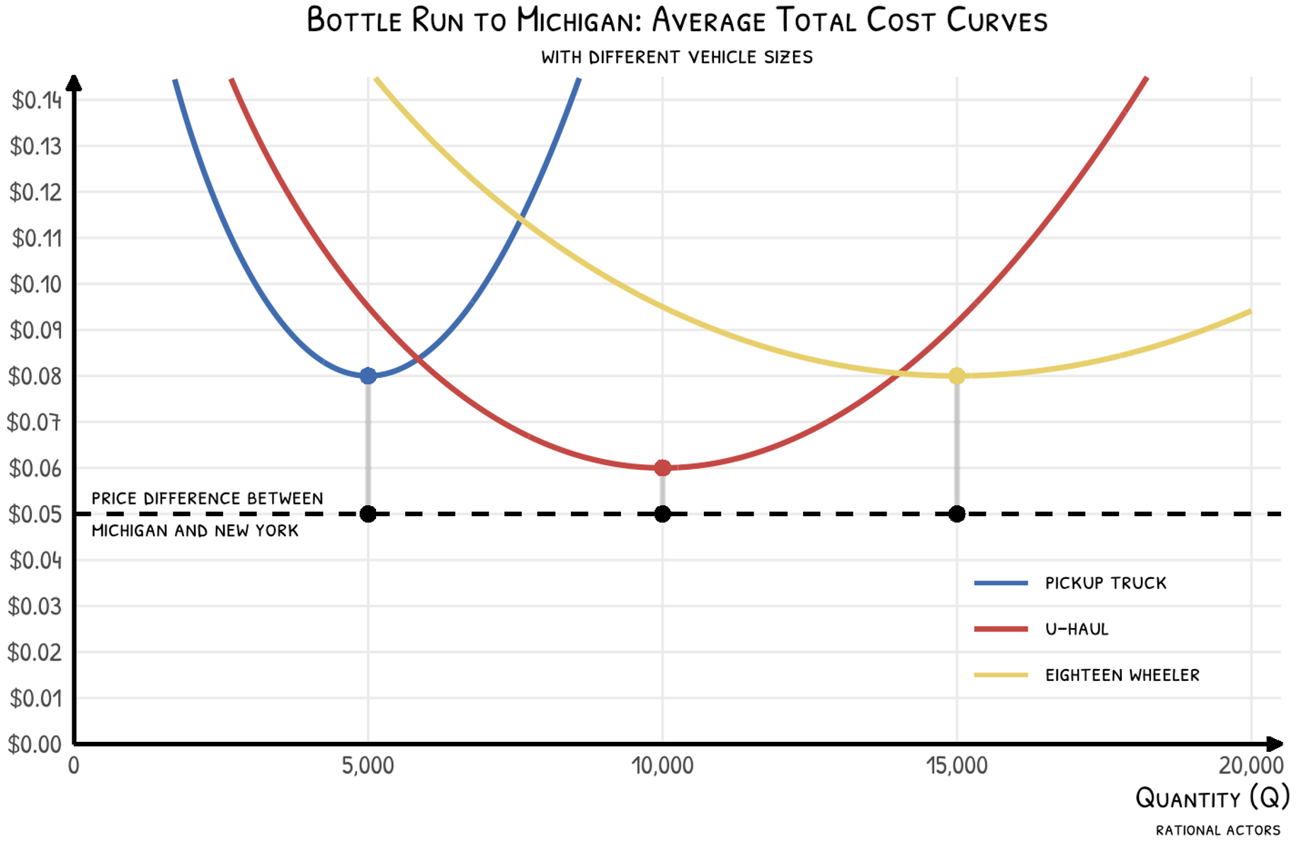
The U-Haul gets close, but none make it to the $0.05 line. Even in a world where the two have no commitment to a particular vehicle and can pick one to suit their needs, it’s still not enough.66 Given that they can freely vary their capital stock, as defined by vehicle size, the graph above creates a long-run average total cost curve. At any quantity, which vehicle size has the lowest average total cost? Use that one. With a continuum of truck sizes, they get a wide, U-shaped long-run average total cost curve that envelops each individual average total cost curve. If the U-Haul achieves the minimum long-run average total cost, then the operation experiences economies of scale from Q = 0 to Q = 10,000 and diseconomies of scale above Q = 10,000: too much overhead.
Then Newman finds a way in. The mother of all mail days is coming up: Mother’s Day. A number of trucks will make their way from New York to Michigan. Newman has signed up for one. For their purposes, it’s as good as free.
Kramer: “A free truck? Oh boy, that completely changes our cost structure. Our G and A goes down fifty percent.”
Newman: “We carry a couple of bags of mail, and the rest is ours!”
This means a precipitous drop in their fixed cost. Even the gas is likely covered by the postal service. The opportunity cost of a couple of days of Kramer’s time is about all that’s lost. This changes the picture entirely.
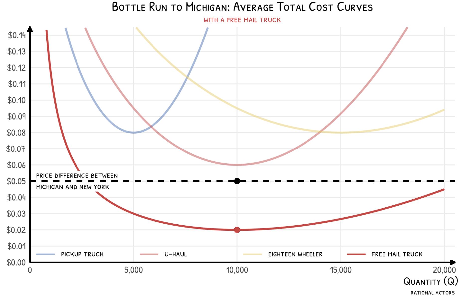
They can be profitable over a wide range of quantities now.77 Based on this model, 10,000 bottles would minimize their average total cost, but it wouldn’t actually maximize their profit. For a few thousand bottles beyond 10,000, marginal cost is still lower than marginal revenue and hauling them would increase profit. As long as they run into no trouble on the road, they’ll make bank by the time they reach Michigan.88 Bringing containers from out of state to collect a refund in Michigan is illegal. Ironically, penalties escalate when 10,000 such bottles or more are deposited.
“Nine thousand, nine hundred and ninety-nine bottles and cans in the trunk, nine thousand, nine hundred and ninety-nine bottles and cans. At ten cents a bottle and ten cents a can, we’re pulling in five hundred dollars a man.”
1 By listing gas as a fixed cost, we’re assuming the bottles are light enough to have no noticeable effect on gas consumption.
2 Marginal cost is the change in total cost from one more bottle. Since fixed cost doesn’t change with additional bottles, marginal cost reflects only changes in variable cost. Mathematically, marginal cost is the derivative of either total or variable cost with respect to quantity.
3 By profit, we mean economic profit, which accounts for opportunity costs. Their scheme could turn an accounting profit without being better than the next-best use of their time.
4 Alternatively, one could model this with the two receiving $0.10 for each bottle in Michigan. The $0.05 they could have received in New York is then added to marginal cost for every bottle transported. The conclusions would be identical.
5 Why relative to average total cost and not average variable cost? They don’t have a truck yet, so their fixed costs are not sunk.
6 Given that they can freely vary their capital stock, as defined by vehicle size, the graph above creates a long-run average total cost curve. At any quantity, which vehicle size has the lowest average total cost? Use that one. With a continuum of truck sizes, they get a wide, U-shaped long-run average total cost curve that envelops each individual average total cost curve. If the U-Haul achieves the minimum long-run average total cost, then the operation experiences economies of scale from Q = 0 to Q = 10,000 and diseconomies of scale above Q = 10,000: too much overhead.
7 Based on this model, 10,000 bottles would minimize their average total cost, but it wouldn’t actually maximize their profit. For a few thousand bottles beyond 10,000, marginal cost is still lower than marginal revenue and hauling them would increase profit.
8 Bringing containers from out of state to collect a refund in Michigan is illegal. Ironically, penalties escalate when 10,000 such bottles or more are deposited.