Good Restaurants Can Fail
The Bear: S2, E3 “Sundae”
Market Power: Monopolistic Competition
Carmen and Sydney are investing all their time and energy into a new upscale restaurant, The Bear. But Sydney gets a reality check when she confronts the fate of other similar Chicago establishments.
“Funkenhausen Joins Growing List of Shuttered Chicago Restaurants”
Restaurants seem like they should be profitable. Their dishes have high markups and many appear packed every night. So why do so many restaurants close and what does it mean for The Bear’s prospects?
Restaurants usually compete in monopolistic competition. In some sense, they have little monopolies on the dishes and service they provide. But there are lots of restaurants and some have very similar offerings. In that sense, it’s the opposite of a monopoly. From a modeling perspective, each restaurant then has a downward-sloping demand curve and the demand for its product is heavily affected by competition.
Will The Bear be profitable in a market like this? To project potential profits, let’s assume that the restaurant sells a single product: a night of service with a tasting menu. Let’s start with an optimistic vision, which Sydney probably has in mind. The Bear’s nightly operations may be modeled as follows:
- Inverse Demand: P = 200 – 0.5Q
- Total Costs: TC = 0.45Q2 + 20Q + 7,000
- Marginal Revenue:11 This is the first derivative of the total revenue function, TR = 200Q – 0.5Q2, with respect to Q. MR = 200 – Q
- Marginal Cost:22 This is the first derivative of the total cost function with respect to Q. MC = 0.9Q + 20
This demand function implies that nobody will pay more than $200 for a meal and 400 people would show up for a free meal. To attract an additional customer, the restaurant must lower its price for all customers. This decreases the impact of additional customers on revenue as the number of customers served each night grows (with further price decreases). The marginal revenue function captures this tradeoff.
This cost structure assumes $7,000 in fixed costs each night along with increasing variable costs as more diners are served. The marginal cost function specifies that to serve one customer would cost about $20 on the margin and each additional meal served gets increasingly costly.
The Bear prices its meals and serves the resulting number of customers by equating marginal revenue and marginal cost. In this optimistic scenario, the outcome is healthy profits every night.
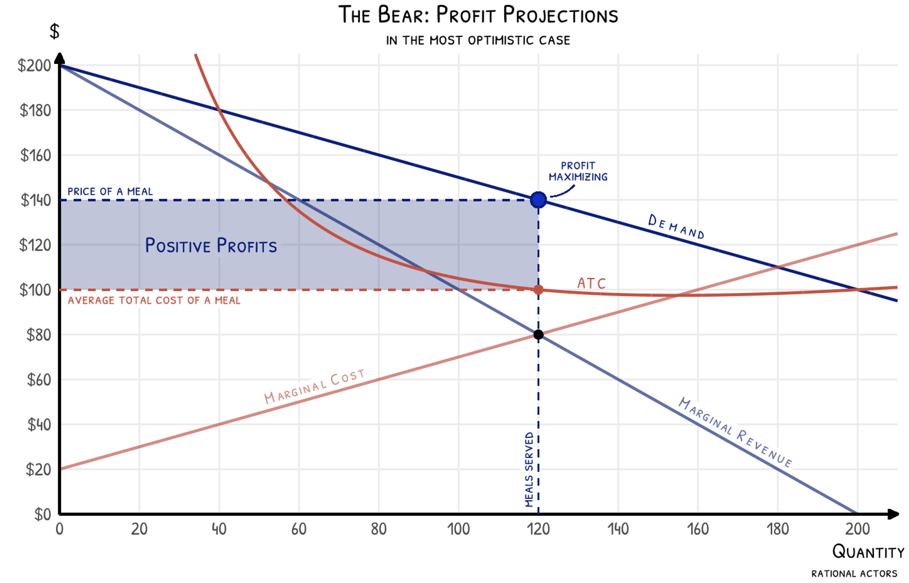
Profit, here, is measured by the difference between price and average total cost multiplied by the quantity of customers served.33 Profit = TR – TC = (TR/Q)*Q – (TC/Q)*Q = P*Q – ATC*Q = (P-ATC)*Q. Each customer pays $140 but the average meal costs only $100 to serve. That’s $40 in profit per customer and $4,800 in profit per night. That would be impressive considering that salary payments to Carmen, Sydney, and compensation to other stakeholders are included in the cost measures here. This outcome is the one the entrepreneurial chefs had in mind.
However, reality begins to set in as The Bear takes shape. Sydney is having trouble on the hiring end. The staff may be more costly than the optimistic projections, raising marginal costs.44 This raises marginal costs because the size of the staff increases as the number of customers served increases. Therefore, higher staff pay makes serving additional customers more costly. Meanwhile, the staff are also overwhelmed by regulatory requirements, so fixed costs are ballooning too.
Sydney: “Did anybody come through?”
Marcus: “Uh, just like 15.”
Sydney: “Oh, looking for jobs?”
Marcus: “Looking for permits.”
Suppose these updated projections raise the marginal cost of serving each meal by $30 and the fixed costs by $500. Now, the results for The Bear are not so rosy.

Here, The Bear passes some of those higher marginal costs on to customers in higher prices, but only $10 worth. Once you account for the higher fixed costs as well, The Bear projects to make zero economic profit. This result is still sustainable. The owners collect a salary and payments to fixed costs, including loan repayments, are covered.
The real trouble for restaurants is that barriers to entry in the industry are not especially high.55 Restaurants have no patent protections, require no specialized licensing beyond basic health and safety permits, and the core product is easily replicated by competitors. In addition, many people dream of opening their own restaurant and are willing to take risks and make sacrifices to try it. They may also have overly optimistic visions. This leads to significant entry with new restaurants frequently popping up. For any individual restaurant, this means greater competition and much more elastic demand for your service despite its uniqueness.66 Here, the demand curve with excess entry has been adjusted to P = 150 – 0.375Q. The same number of customers show up for a free meal, but now the choke price of demand is $150. Demand for any one product becomes more elastic as the number of close substitutes increases.

Once you factor in excessive entry of competing restaurants, it becomes a straightforward path to negative profits. In this pessimistic scenario, The Bear still sells its meals with a markup, but it no longer collects enough nightly revenue to cover total costs.77 A restaurant in this position maximizes profit by continuing to operate if total revenue exceeds variable costs, since nightly fixed costs are sunk. In this example, nightly revenue is $9,600 and variable costs are $6,880. The Bear would only shut down in the long run when fixed costs become variable costs. That might happen when leases expire and need to be renewed or other fixed commitments become possible to get out of. The more elastic demand brought about by competition depresses its prices and reduces its customer base.
Many restaurants meet this exact same fate. They are pulled down by other overly optimistic entrants. Yet the new restaurants keep popping up despite the cautionary tales. The Bear is one of those entrants. Hopefully, at the very least, Carmen and Sydney have everything buttoned up on the financial side of things.
Sydney: “But you had a restaurant before, right?”
Chef: “Yeah, my wife and I had a restaurant in Bucktown.”
Sydney: “Why do you think it closed?”
Chef: “We had a terrible business partner who took all of our money and flew off to Hawaii. I wish that wasn’t a common story in this business, but, you know, these things happen all the time.”
1 This is the first derivative of the total revenue function, TR = 200Q – 0.5Q2, with respect to Q.
2 This is the first derivative of the total cost function with respect to Q.
3 Profit = TR – TC = (TR/Q)*Q – (TC/Q)*Q = P*Q – ATC*Q = (P-ATC)*Q.
4 This raises marginal costs because the size of the staff increases as the number of customers served increases. Therefore, higher staff pay makes serving additional customers more costly.
5 Restaurants have no patent protections, require no specialized licensing beyond basic health and safety permits, and the core product is easily replicated by competitors.
6 Here, the demand curve with excess entry has been adjusted to P = 150 – 0.375Q. The same number of customers show up for a free meal, but now the choke price of demand is $150. Demand for any one product becomes more elastic as the number of close substitutes increases.
7 A restaurant in this position maximizes profit by continuing to operate if total revenue exceeds variable costs, since nightly fixed costs are sunk. In this example, nightly revenue is $9,600 and variable costs are $6,880. The Bear would only shut down in the long run when fixed costs become variable costs. That might happen when leases expire and need to be renewed or other fixed commitments become possible to get out of.